As you probably already know, the Excel VBA match function looks for the position or row number of the lookup value in the table array which is the same as saying, in the main excel table.
Some of the most popular lookup functions include VLOOKUP, HLOOKUP, MATCH, INDEX, among others. While there are some more important (or more used) than others, the reality is that these same functions simply aren’t available in VBA. The good news is that you can still use the same functions that are available as worksheet functions under the VBA script to make your life a lot easier.
So, to give you a better idea of how this works, we decided to tell you a bit more about the Excel VBA match function today.
Learn about rounding numbers here.
The Excel VBA Match Function
As you can easily understand, the VBA Match has the same use as the Match formula in Excel.
Notice that this function finds a match within an array with reference to the lookup value and prints its position.
One of the main benefits of using the Excel VBA match index is the fact that it can be very useful when you are trying to evaluate your data based on certain values. For example, this function can be useful when you have the salary data of your employees and you need to discover the numeric position of an employee in your data to see who has a salary less than, greater than, or equal to a specific value. As you can see, this insight can be pretty helpful and it only takes you a line of code.
Understanding the Excel VBA round function.
The Syntax Of The Excel VBA Match Function
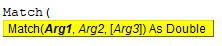
Where,
- Arg1 – Lookup_value – The value you need to lookup in a given array.
- Arg2 – Lookup_array – an array of rows and columns which contain possible Lookup_value.
- Arg3 – Match_type – The match type which takes value -1, 0, or 1.
- When the match_type = -1, this means that the Match function will find out the smallest value which is greater than or equals to the lookup_value. For this to happen, the lookup_array must be sorted in descending order.
- When the match_type = 0, it means that the Match function will find out the value which is exactly the same as that of the lookup_value.
- When the match_type = +1, it means that the Match function will find out the largest value which is lesser than or equals to the lookup_value. For this to happen, the lookup_array must be sorted in ascending order. The default value for the match type is +1.
How To Use The Excel VBA Match Function
In order to use this function, you just need to follow the next steps.
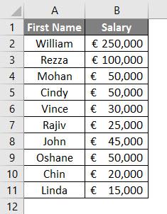
The goal of this example is to discover who from this list has a salary of €30,000 along with position in Excel.
The reality is that we could easily determine this by hand since we have small data. However, the point is for you to understand how to use this function.
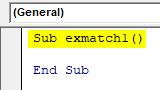
Step #1: Define a sub-procedure by giving a name to macro.
Let’s say that you define the code:
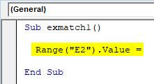
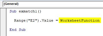
Step #2: At this point, you want your output to b stored in cell E2. So, you just need to write the code as Range(“E2”).Value =
If you think about it, this simply defines the output range for your result.
Check out the rules for rounding fractions.
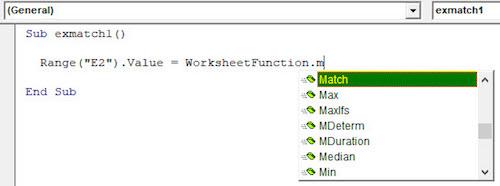
Step #3: Now it’s time to use the Excel VBA match function.
Step #4: Use the code:
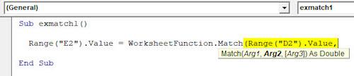
Step #5: Now, you need to give arguments to the MATCH function such as the Lookup_value. Our Lookup_value is stored in cell D2 as shown in the below screenshot.
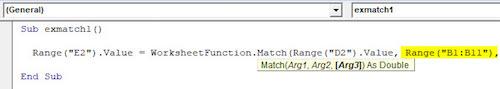
Step #6: The second argument is Lookup_array. This is the table range within which you want to find out the position of Lookup_value. In our case, it is (B1:B11). Provide this array using the Range function.
Use our simple calculator to round your numbers to the nearest tens.
Step #7: The Last argument for this code to work out is Match_type. We wanted to have an exact match for Lookup_value in given range> Therefore, give Zero (0) as a matching argument
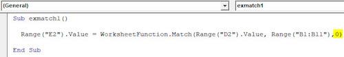
Step #8: Run this code by hitting F5 or Run button and see the output.
You can see in Cell E2, there is a numeric value (6) which shows the position of the value from cell D2 through range B1:B11.