One of the most popular functions in Excel is the SUMIF function. After all, it allows you to perform a wide range of calculations in an easy and practical way instead of taking a lot of time if you were performing them by hand.
Discover everything you need to know about rounding numbers.
What Is The SUMMIF Function?
Simply put, the SUMIF function in excel is a simple function that returns the sum of cells that meet a specific condition.

One of the things that many people don’t know about the SUMIF function in excel is that it can be applied to numbers, text, and even dates.
It is also important to keep in mind that the SUMIF function supports logical operators (>,<,<>,=) as well as wildcards (*,?) for partial matching.
The main goal to use this function is to sum numbers in a range that meets all your criteria.
Looking to round decimals to the nearest whole number?
The Syntax Of The SUMIF Function
When you are looking to add the SUMIF function, you need to express it in the following way:
=SUMIF (range, criteria, [sum_range])
And here are the arguments:
- Range: This refers to the range of the cells that you want to apply the criteria against.
- Criteria: This is the criteria that you define and that will be used to determine which cells to add.
- Sum_range: This argument is optional and when you don’t specificy it, it will assume that the cells in the range are added together. In case you want, you can specify the cells that you need to add together.
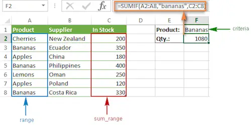
While you probably already understand all these arguments, it is important to notice that the SUMIF function returns the sum of cells in a range that meet a single condition. The first argument is the range to apply criteria to, the second argument is the actual criteria, and the last argument is the range containing values to sum.
In addition, the SUMIF supports logical operators (>,<,<>,=) and wildcards (*,?) for partial matching. If you need to apply more than one criteria, you should then use the SUMIFS function.
As we already mentioned above, you can use this function with numbers, text, and even dates. Let’s take a closer look at each one of these.
Why you need to know how to round numbers?
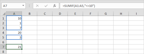
#1: SUMIF Function With Numeric Criteria:
Let’s say that you want to use the SUMIF function that has two arguments below. As you can see, it sums values in the range A1:A5 that are less than or equal to 10.
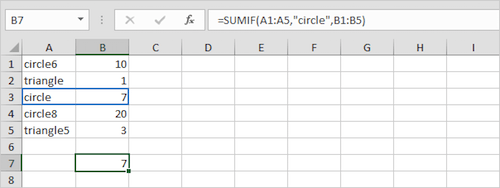
#2: SUMIF Function With Text Criteria:
While this may seem a bit strange since we are talking about sums, the truth is that you may need to get all the cells with text that meet a specific criteria. However, you need to ensure that you always enclose the text in double quotation marks. In addition, you will be glad to know that you can also use wildcards.
Here’s an example of the SUMIF function that sums values in the range B1:B5 if the corresponding cells in the range A1:A5 exactly contain circle:
Discover how you can round numbers up in Excel.
#3: SUMIF Function With Date Criteria:
Just like numeric or text criteria, you can also use date criteria in your SUMIF function.
Here’s an example. As you can see, the SUMIF function below sums the sales after January 20th, 2018:
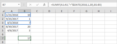
It is important to notice that the date function accepts 3 arguments: year, month, and day.